Weighted Average in SQL: Examples, Formulas, and Best Practices (2025 Guide)

When analyzing data, a simple average often isn’t enough. Some values matter more than others, and treating every record equally can lead to misleading insights. That’s where the weighted average in SQL comes in.

A SQL weighted average often shows up in reporting and analytics, whether it’s finding a customer’s average order value adjusted for quantity, calculating GPA from course units, or analyzing revenue per region based on sales volume. Unlike the simple average, which treats every record equally, the weighted average makes sure each value contributes in proportion to its significance.

In this guide, we will explore weighted average SQL: the formulas, step-by-step query examples, and best practices for real-world use cases.

A weighted average is a way of calculating an average where some values count more than others. Instead of treating every value the same, you give more “weight” to values that are more important (such as sales quantities, course units, or frequencies).

Weighted Average Formula

The formula for weighted average is:

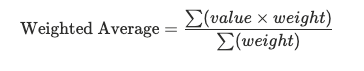
• Value = the number you’re measuring (e.g., price, score, revenue).
• Weight = the factor that adjusts its importance (e.g., quantity, units, frequency).

For example:

• Grade 1 = 90 with 3 units
• Grade 2 = 80 with 2 units

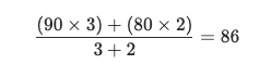
Here, the 3-unit class has a bigger effect on the final average than the 2-unit class.

Simple Average vs Weighted Average in SQL

In SQL, a simple average uses the AVG() function, which adds up all values and divides by the number of rows. Every row is treated equally. A weighted average multiplies each value by its weight, sums the results, and then divides by the total weight. This way, rows with larger weights have a bigger impact on the final result.

A weighted average in SQL is often calculated using the SUM/Weight method. You multiply each value by its weight, add the results together, and then divide by the total weight.

SQL Formula

The general SQL weighted average formula looks like this:

SELECT SUM(value * weight) / SUM(weight) AS weighted_avg
FROM your_table;

• value is the column you want to average (e.g., grade, price, or revenue).
• weight is the column that defines importance (e.g., units, quantity, or frequency).

Common Use Case: GPA Calculation

A classic case is calculating a student’s GPA, where each grade has a weight based on course units:

SELECT SUM(grade * units) / SUM(units) AS gpa
FROM student_grades;

• grade = the student’s score
• units = the course weight

In this query, a 3-unit course pulls the GPA weighted average in SQL more strongly than a 1-unit course.

When working with real-world data, you often need to calculate weighted averages across categories or after joining multiple tables. This is where mistakes happen. If you simply use AVG() or forget to handle duplicates created by a join, you can end up with the wrong numbers. Knowing how to calculate weighted average correctly with GROUP BY and JOIN is key.

Avoiding Incorrect Averages After Joins

A common mistake is joining tables and then using AVG(). For example, joining orders and order_items may create duplicate rows. If you calculate a weighted average directly on this joined data, the result will not be accurate.

Always identify the column that represents the weight, such as quantity or units, and use it in your calculation instead of relying on the joined rows.

Correct Query Pattern With GROUP BY

The correct way is to multiply each value by its weight, sum the results, and then divide by the total weight. Use GROUP BY when you want the weighted average per category.

Example: Weighted average sales price per customer:

SELECT 
    customer_id,
    SUM(price * quantity) / SUM(quantity) AS weighted_avg_price
FROM order_items
GROUP BY customer_id;

• price is the value
• quantity is the weight
• customer_id is the category

Weighted averages are not always static. In time series or sequential data, you may need a running total or a moving window to see how values change over time. SQL lets you handle these cases with window functions and date logic. Knowing how to calculate a running weighted average or a weighted rolling average is especially useful in sales reports, financial metrics, and performance tracking.

Running Weighted Average With Window Functions

A running weighted average shows the cumulative average up to each point in time. You can do this with a window function.

Example: Running weighted average sales price by date:

SELECT
    sale_date,
    SUM(price * quantity) OVER (ORDER BY sale_date ROWS BETWEEN UNBOUNDED PRECEDING AND CURRENT ROW)
      / SUM(quantity) OVER (ORDER BY sale_date ROWS BETWEEN UNBOUNDED PRECEDING AND CURRENT ROW) 
      AS running_weighted_avg
FROM sales;

• price is the value
• quantity is the weight
• The window function calculates the cumulative sums up to the current date.

Rolling Weighted Moving Average

A weighted rolling average looks at a fixed time window, such as the last 3 days. This is useful for smoothing out short-term spikes and trends.

Example: 3-day weighted moving average of sales:

SELSELECT
    sale_date,
    SUM(price * quantity) OVER (ORDER BY sale_date ROWS BETWEEN 2 PRECEDING AND CURRENT ROW)
      / SUM(quantity) OVER (ORDER BY sale_date ROWS BETWEEN 2 PRECEDING AND CURRENT ROW) 
      AS rolling_weighted_avg
FROM sales;

Handling Missing Dates in Time Series

When working with time series data, missing dates can cause gaps in your averages. For example, if no sales happened on a certain day, that date won’t appear in your table.

To fix this, create a calendar table or generate a series of dates, then join it with your sales data. That way, every date is included, even if sales are zero. After filling in missing dates, your moving average SQL query will produce smoother and more accurate results.

The logic for calculating a weighted average is the same everywhere: multiply values by weights, sum the results, and divide by the total weight. However, SQL syntax can look slightly different depending on the database. Below are examples of how to write a weighted average in Postgres, Snowflake, SQL Server, and MySQL.

Postgres Weighted Average Example

In PostgreSQL, the formula can be written directly in a SELECT statement:

SELECT SUM(price * quantity) / SUM(quantity) AS weighted_avg_price
FROM sales;

The syntax looks the same as other databases. The difference is that Postgres allows the FILTER clause inside aggregates, which makes conditional weighted averages easier:

SELECT
  SUM(price * quantity) FILTER (WHERE region = 'East')
  / SUM(quantity) FILTER (WHERE region = 'East') AS east_weighted_avg
FROM sales;

Snowflake Weighted Average Example

Snowflake also uses the same base query but what makes Snowflake different is its strong support for window functions and handling time-series data. For example, you can calculate a running weighted average by date:

SELECT
    PRODUCT_ID,
    SUM(SALES_AMOUNT * QUANTITY_SOLD) / SUM(QUANTITY_SOLD) AS WEIGHTED_AVERAGE_SALES_PER_PRODUCT
FROM
    SALES_DATA
GROUP BY
    PRODUCT_ID
ORDER BY
    PRODUCT_ID;

The weighted average is cumulative, using all grades and course units up to the current term.

SQL Server Weighted Average Example

The syntax is the same as Postgres and Snowflake. The difference is that SQL Server developers often rely on Common Table Expressions (CTEs) to break down multi-step weighted average calculations. For example, calculating by region:

WITH regional_sales AS (
  SELECT region, price, quantity
  FROM sales
)
SELECT 
  region,
  SUM(price * quantity) / SUM(quantity) AS weighted_avg_price
FROM regional_sales
GROUP BY region;

MySQL Weighted Average Example

In MySQL 8 and above, the syntax is also the same. The difference is in version support. Modern MySQL supports window functions, so you can also do running or rolling weighted averages:

SELECT
    student_id,
    SUM(score * weight) / SUM(weight) AS weighted_average_score
FROM
    grades
GROUP BY
    student_id;

Weighted averages are more than just theory; they are used in actual school, marketing, and sales decisions. Here are a few examples where the weighted average formula is more accurate than a simple average.

Weighted Average Email Campaign

Clicks usually matter more than opens. By weighting clicks at 0.7 and opens at 0.3, marketers can calculate a single score that better reflects campaign effectiveness.

SELECT 
  campaign_id,
  ROUND(
    (0.3 * AVG(open_rate) + 0.7 * AVG(click_rate)), 
    2
  ) AS weighted_avg_score
FROM email_campaigns
GROUP BY campaign_id;

Weighted Sales Performance

To spot trends without daily spikes, sales teams use a weighted moving average that gives higher weight to recent days and less to earlier ones.

SELECT
  product_id,
  sale_date,
  ROUND(
    0.5 * sales
    + 0.3 * LAG(sales, 1) OVER (PARTITION BY product_id ORDER BY sale_date)
    + 0.2 * LAG(sales, 2) OVER (PARTITION BY product_id ORDER BY sale_date),
    2
  ) AS weighted_moving_avg
FROM sales
WHERE LAG(sales, 2) OVER (PARTITION BY product_id ORDER BY sale_date) IS NOT NULL;

Weighted averages are powerful, but there are common mistakes and performance traps to watch out for. Handling them well ensures your results are accurate and your queries run efficiently.

Handling NULLs and Zero Weights

If either the value or the weight is NULL, the multiplication returns NULL and can skew the result. Use COALESCE to replace NULL with zero:

SUM(COALESCE(value, 0) * COALESCE(weight, 0)) / NULLIF(SUM(weight), 0)

Also watch out for cases where the total weight is zero. Dividing by zero will cause an error, so wrapping it with NULLIF(SUM(weight), 0) prevents the issue.

Precision and Rounding Issues

Weighted averages often involve decimal calculations. Small rounding errors can add up when working with large numbers or financial data. To keep results precise:

• Use the right data type (e.g., DECIMAL instead of FLOAT).
• Apply ROUND() only at the final step, not inside calculations.

Performance Considerations on Large Tables

On large datasets, repeated calculations of value * weight can be expensive. A few tips:

• Pre-aggregate in Common Table Expressions (CTEs) or temp tables before joining.
• Add indexes on join keys and ORDER BY columns if using window functions.
• For frequent queries, consider storing precomputed weighted averages in summary tables.

What is the difference between simple and weighted average in SQL?

A simple average treats every row equally; it just adds values and divides by the count. A weighted average multiplies each value by a weight, then divides by the total weight, so rows with higher importance contribute more.

Can you calculate a moving average in SQL?

Yes. You can use window functions like AVG() with ROWS BETWEEN for a simple moving average. For a weighted moving average, combine window functions with weights (value * weight / SUM(weight)) to give recent rows more influence.

What’s the difference between weighted sum vs weighted average?

A weighted sum is just the total of values multiplied by their weights. A weighted average divides that weighted sum by the total weight. Without dividing, the result is a sum, not an average.

How do you calculate weighted average in Postgres/Snowflake?

Both databases use the same formula:

SELECT SUM(value * weight) / SUM(weight) AS weighted_avg
FROM table_name;

Postgres offers a FILTER clause that makes conditional weighted averages easier. Snowflake is strong with analytic functions, which are great for running or rolling weighted averages.

What happens if weights are zero or NULL in SQL?

If weights are NULL, the calculation may return NULL. If the total weight is zero, dividing by zero will cause an error. To avoid this, use COALESCE to handle NULL values and NULLIF(SUM(weight), 0) to prevent division errors.

A weighted average in SQL gives you more accurate insights than a simple average because it accounts for the importance of each value. Whether you are calculating GPA, measuring sales performance, or analyzing marketing campaigns, the approach is the same: multiply values by weights, sum them up, and divide by the total weight.

Always be mindful of edge cases like NULLs, zero weights, and large datasets where performance matters. With the right formulas and best practices, you can apply weighted averages confidently across different SQL dialects and real-world business problems.

• SQL Conditional Join
• SQL Cumulative Sum
• SQL Left Join To Combine Multiple Rows

For interview preparations, check out the following:

• SQL Interview Questions
• Data Analytics Project Ideas
• Analytic Functions in SQL Guide