SQL JOIN on Multiple Columns Cheat Sheet: Syntax & Examples

In SQL, a JOIN combines rows from two or more tables based on a related column. It’s a core technique in querying normalized databases. But in real-world scenarios, joining on a single column often isn’t enough.

This guide is a practical, 2025-ready walkthrough of SQL joins on multiple columns—what they are, when to use them, and how to write them correctly across INNER, LEFT, RIGHT, and FULL joins.

You’ll learn to spot real situations that demand composite keys, avoid common pitfalls, and improve performance with composite indexes and execution plans.

We include clear syntax patterns for major dialects (MySQL, PostgreSQL, SQL Server, Oracle), side-by-side examples, and troubleshooting tips so you can move from “it works” to “it’s correct and fast.”

By the end, you’ll have a repeatable toolkit to prevent duplicate blowups, ensure accurate matches, and confidently tackle multi-column joins in interviews and real production workloads.

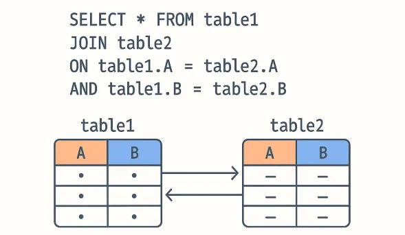
In SQL, a JOIN on multiple columns means that two or more conditions must be satisfied for rows to match between tables. Instead of joining on a single key (like id), you specify multiple keys in the ON clause by combining them with AND. In simple terms, a JOIN on multiple columns means you’re telling SQL: Only connect these two rows if more than one thing matches.

When Would You Actually Use This? (Timing in Real Work)

1. When one column is not unique enough: For example, an employee_first_name may appear many times. You need both first_name and last_name to reliably join.
2. When data is recorded at multiple levels: Daily sales data often uses both store_id and sale_date — you wouldn’t want to match a store’s sales from the wrong day.
3. When a key is made of two or more parts (composite key): In some databases, the “primary key” is a combination of columns (like region_id + store_id). Whenever you query those tables, you need to join on both to get the right match.

Real-World Use Cases

Use Case	Columns to Join	Why
Matching sales by store and date	store_id, sale_date	Aligns daily sales across systems; prevents cross-store or cross-day mismatches.
Identifying employees by first and last name	first_name, last_name	Provides a composite identifier when a unique employee ID isn’t available.
Combining region and store IDs for reporting	region_id, store_id	Ensures accurate joins between fact and dimension tables for rollups and reporting.

When working with SQL, you can extend any type of join to match on more than one column. This is done by chaining JOIN conditions in the ON clause with the AND operator. Let’s look at how this works across different join types.

INNER JOIN on Multiple Columns

The INNER JOIN only returns rows that satisfy all join conditions. This is the most common use case when combining tables with composite keys.

SELECT a.*, b.*
FROM orders a
INNER JOIN shipments b
  ON a.order_id = b.order_id
 AND a.customer_id = b.customer_id;

Here, a row is returned only if both order_id and customer_id match between the orders and shipments tables.

LEFT JOIN on Multiple Columns

A LEFT JOIN ensures that all rows from the left table appear in the result, even if no match is found on one or more join conditions. If no match exists, the right-side columns will contain NULL.

SELECT a.*, b.*
FROM employees a
LEFT JOIN payroll b
  ON a.emp_first = b.emp_first
 AND a.emp_last = b.emp_last;

This allows you to keep all employees, even those not yet entered into the payroll system.

RIGHT/FULL OUTER Joins on Multiple Columns

While less common, you can also apply multiple-column conditions to RIGHT JOIN or FULL OUTER JOIN. These joins help capture non-matching rows from one or both sides.

SELECT a.*, b.*
FROM regions a
FULL OUTER JOIN stores b
  ON a.region_id = b.region_id
 AND a.division_id = b.division_id;

This query ensures you see all regions and all stores, even if some combinations don’t have a perfect match.

Remember: Adding multiple conditions makes the join stricter. Rows will only align if every specified column matches. If one column mismatch occurs, the join result depends on the join type (INNER, LEFT, RIGHT, FULL).

Sometimes a single column isn’t enough to guarantee the right match. Imagine we’re working with employee data. Both the employees and salaries tables use employee_id, but in this company, IDs are reused across departments. That means if you join only on employee_id, you’ll run into duplicate or mismatched rows.

employees table:

employee_id	first_name	department
101	Alice	Sales
101	Bob	Marketing
102	Carol	HR

salaries table:

employee_id	department	salary
101	Sales	70,000
101	Marketing	65,000
102	HR	60,000

The Problem: Joining on a Single Column

SELECT e.employee_id, e.first_name, e.department, s.salary
FROM employees e
JOIN salaries s
  ON e.employee_id = s.employee_id;

Incorrect Output

employee_id	first_name	department	salary
101	Alice	Sales	70,000
101	Alice	Sales	65,000
101	Bob	Marketing	70,000
101	Bob	Marketing	65,000
102	Carol	HR	60,000

Because the join only checks employee_id, Alice and Bob’s rows get tangled up with both salary records.

How to Fix This: Joining on Multiple Columns

SELECT e.employee_id, e.first_name, e.department, s.salary
FROM employees e
JOIN salaries s
  ON e.employee_id = s.employee_id
 AND e.department = s.department;

Correct Output

employee_id	first_name	department	salary
101	Alice	Sales	70,000
101	Bob	Marketing	65,000
102	Carol	HR	60,000

By joining on both employee_id and department, SQL ensures that each employee only matches the salary data from their department. This avoids mismatches, keeps results accurate, and mirrors how real-world databases often use composite keys (two or more fields together uniquely identify a row).

Test your skills with real-world challenges from top companies to cement concepts before the interview.

Once you’re comfortable with basic two-column joins, you’ll often encounter more advanced scenarios in real-world SQL work. These go beyond simple equality matches and require careful attention to logic and data quality.

Three-Column JOINs (SQL Server Example)

Sometimes two columns still aren’t enough. In cases where uniqueness depends on three fields, you can extend the join condition further.

SELECT a.*, b.*
FROM orders a
JOIN shipments b
  ON a.order_id = b.order_id
 AND a.customer_id = b.customer_id
 AND a.ship_date = b.ship_date;

Here, all three conditions must hold true. This is common when the combination of order, customer, and date uniquely identifies a transaction.

Range JOINs (Date Overlaps)

Not all joins are based on exact equality. A range join links rows when a value falls between two endpoints, which is commonly used for date ranges.

SELECT e.employee_id, e.start_date, e.end_date, p.project_name
FROM employees e
JOIN projects p
  ON e.start_date BETWEEN p.start_date AND p.end_date;

This matches employees to projects if their start date falls within the project’s timeline. Range joins are powerful in scheduling, time tracking, or booking systems.

JOINs with Different Column Names

Tables often store the same concept under different column names. You can still join them by explicitly matching across names.

SELECT a.colA, b.colX
FROM table_a a
JOIN table_b b
  ON a.colA = b.colX;

For example, customer_id in one table may be stored as client_id in another. What matters is the values, not the column names.

Joining with NULL Values (Pitfalls)

A tricky case arises when the join columns can contain NULL. By default, NULL = NULL evaluates to false, so those rows won’t match.

SELECT a.*, b.*
FROM contracts a
JOIN renewals b
  ON a.client_id = b.client_id
 AND a.optional_code = b.optional_code;

If optional_code is NULL in both tables, this row won’t appear in the results. To handle this, you may need IS NULL conditions or functions like COALESCE:

ON COALESCE(a.optional_code, 0) = COALESCE(b.optional_code, 0)

This treats missing values as equal stand-ins, preventing data loss in joins.

While multi-column joins are powerful, they also come with some common mistakes and performance challenges. Being aware of these issues can save you from messy results and slow queries.

Forgetting a JOIN Condition

The most frequent error is leaving out one of the required columns in the ON clause. For example, joining only on employee_id but forgetting to also join on department can multiply rows and create mismatches. Always double-check that every column needed for uniqueness is included in the join condition.

Symptom: Duplicate/mismatched rows because not all key parts are in the ON clause.

Optimization Tip: Join on the full composite key; validate row counts before/after.

Wrong

-- Missing store_id in the join: orders will multiply across stores
SELECT o.order_id, s.shipment_id
FROM orders o
JOIN shipments s
  ON o.order_id = s.order_id;  -- ❌ forgot o.store_id = s.store_id

Corrected

SELECT o.order_id, s.shipment_id
FROM orders o
JOIN shipments s
  ON o.order_id = s.order_id
 AND o.store_id  = s.store_id;  -- ✅ complete composite match

Data Type Mismatches

If the columns you’re joining on don’t share the same data type, say one is CHAR(5) and the other is VARCHAR(5)then SQL may still run the query but will need to implicitly convert data. This not only risks mismatches (due to padding or trimming) but also slows performance. Ensuring consistent data types across join keys is a best practice.

Symptom: Slow joins or mismatches (implicit casts), e.g., CHAR vs VARCHAR, INT vs TEXT.

Optimization Tip: Normalize types ahead of time; cast explicitly if you must.

Bad (implicit cast at runtime)

-- o.dept_id is INT, e.dept_id is TEXT; engine must cast per row
SELECT e.emp_id, o.role
FROM employees e
JOIN org_map o
  ON e.dept_id = o.dept_id;  -- ❌ type mismatch causes implicit casting

Better (explicit cast)

-- Use explicit, sargable casting where possible
SELECT e.emp_id, o.role
FROM employees e
JOIN org_map o
  ON e.dept_id = CAST(o.dept_id AS INT);

Best (schema-aligned)

-- Align types in schema or a prep step
ALTER TABLE org_map
  ALTER COLUMN dept_id TYPE INT USING dept_id::INT;  -- Postgres example

Performance Issues Without Composite Indexes

When you join on multiple columns, the database engine performs better if there’s a composite index (an index covering all of the join columns in order). Without it, the query optimizer may resort to full table scans, which can be slow on large datasets. If you frequently join on (col1, col2), consider adding an index on both together rather than separately.

Symptom: Full scans / hash joins on big tables; poor latency and high cost.

Optimization Tip: Add a composite (covering) index in the join column order most used by filters and joins.

Before

-- Joins on (customer_id, order_date) but only single-column indexes exist
SELECT o.*, f.flag
FROM orders o
JOIN fraud_flags f
  ON o.customer_id = f.customer_id
 AND o.order_date  = f.order_date
WHERE o.order_date >= CURRENT_DATE - INTERVAL '30 days';

After (Postgres syntax; adapt for your DB)

-- Composite index supports the join and the date predicate
CREATE INDEX idx_orders_cust_date ON orders (customer_id, order_date);
CREATE INDEX idx_flags_cust_date  ON fraud_flags (customer_id, order_date);

-- Same query benefits from index lookups/merge/hash with far fewer scans
SELECT o.*, f.flag
FROM orders o
JOIN fraud_flags f
  ON o.customer_id = f.customer_id
 AND o.order_date  = f.order_date
WHERE o.order_date >= CURRENT_DATE - INTERVAL '30 days';

Rule of Thumb: If you frequently join/filter on (col1, col2), prefer one composite index (col1, col2) over two separate indexes.

Using Execution Plans for Debugging

If a multi-column join runs slowly, use EXPLAIN (MySQL, PostgreSQL) or query execution plans (SQL Server, Oracle) to see how the database is handling it. These tools show whether indexes are being used, if full scans are happening, and which join algorithms (nested loop, hash join, merge join) are in play. Optimizing based on this insight can make a huge difference in performance.

Symptom: Guesswork tuning; hidden bottlenecks (bad join order, spills, full scans).

Optimization Tip: Inspect the plan (EXPLAIN, EXPLAIN ANALYZE) to see join type, index usage, and row estimates, then tune accordingly.

Postgres Example

EXPLAIN ANALYZE
SELECT a.*, b.attr
FROM dim_accounts a
JOIN fact_events b
  ON a.account_id = b.account_id
 AND a.region     = b.region
WHERE b.event_ts >= NOW() - INTERVAL '7 days';

What to look for

• JOIN type: Nested Loop vs Hash vs Merge (pick the cheapest for your data size/distribution).
• Index usage: Ensure the composite indexes on (account_id, region) exist and are used.
• Row estimates: Big estimate errors → consider updating stats or rewriting predicates.
• I/O & memory: Look for large hash tables or sorts; add indexes or adjust work memory if warranted.

Targeted Fix (if plan shows scans on fact table)

-- Help the join + filter
CREATE INDEX idx_fact_events_acct_region_ts
  ON fact_events (account_id, region, event_ts DESC);

Although the concept of joining on multiple columns is universal, each SQL dialect offers small differences in syntax, optimization strategies, and indexing behavior. Knowing these differences can help you write cleaner, faster queries tailored to the database you’re working with.

MySQL

In MySQL, the standard ON col1 = col1 AND col2 = col2 syntax applies. Performance benefits come from properly defining composite indexes on the join columns. Without them, MySQL may resort to table scans. You can also use EXPLAIN to verify whether indexes are being picked up, which is especially important on large datasets.

SELECT o.order_id, o.customer_id, s.shipment_date
FROM orders o
JOIN shipments s
  ON o.order_id = s.order_id
 AND o.customer_id = s.customer_id;

PostgreSQL

PostgreSQL supports the same multi-column join syntax but shines when you leverage composite indexes. An index like CREATE INDEX idx_orders_customer_date ON orders(customer_id, order_date); helps PostgreSQL quickly filter and match rows. Its EXPLAIN ANALYZE command goes deeper than MySQL’s EXPLAIN, giving actual run-time stats for fine-tuning join performance.

-- Same join, plus composite index for performance
CREATE INDEX idx_orders_customer_date
  ON orders (customer_id, order_date);

SELECT o.customer_id, o.order_date, p.payment_status
FROM orders o
JOIN payments p
  ON o.customer_id = p.customer_id
 AND o.order_date  = p.order_date;

Oracle

Oracle SQL allows the usual ON a.col1 = b.col1 AND a.col2 = b.col2 but also supports a shorthand with the USING clause when the column names are identical:

SELECT *
FROM employees e
JOIN salaries s
  USING (employee_id, department);

This makes the query cleaner by avoiding repeated column names, though it only works when the join columns have the same name in both tables.

SQL Server

SQL Server follows the same multi-column join syntax as MySQL and PostgreSQL but offers optimization tricks like indexed views and detailed execution plans through SQL Server Management Studio (SSMS). The optimizer can sometimes choose hash joins, merge joins, or nested loops depending on available indexes. Defining composite keys and using clustered indexes on frequently joined columns helps SQL Server scale better for multi-column joins.

SELECT o.order_id, o.customer_id, s.shipment_date
FROM dbo.orders o
JOIN dbo.shipments s
  ON o.order_id = s.order_id
 AND o.customer_id = s.customer_id;

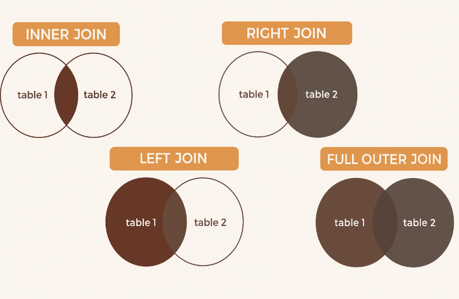
To make the difference concrete, imagine two filters in series. With a single-column join, rows match when one attribute lines up (e.g., store_id). With a multi-column join, the row must pass through both filters (e.g., store_id and sale_date).

Conceptually, that’s the shift from a broad overlap to a narrower intersection: first you line up by store, then you keep only the rows that also share the same date. This mental model helps explain why multi-column joins reduce accidental matches and duplicate inflation since fewer rows satisfy all conditions.

A quick cross-dialect view also clarifies how the syntax stays consistent while conveniences vary. MySQL and PostgreSQL typically rely on the classic ON a.col1 = b.col1 AND a.col2 = b.col2 form, while Oracle adds a USING shorthand when column names are identical in both tables. SQL Server shares the same ON ... AND ... pattern and is often tuned with composite (and sometimes clustered) indexes on the join keys.

Syntax at a Glance (by Dialect)

Dialect	Typical Equality Join on Two Columns	Notes
MySQL	... JOIN b ON a.c1 = b.c1 AND a.c2 = b.c2	Use EXPLAIN to confirm composite-index usage.
PostgreSQL	... JOIN b ON a.c1 = b.c1 AND a.c2 = b.c2	EXPLAIN ANALYZE gives actual timings; composite indexes matter.
Oracle	... JOIN b USING (c1, c2)	USING only when column names match on both sides; otherwise use ON.
SQL Server	... JOIN b ON a.c1 = b.c1 AND a.c2 = b.c2	Inspect plans in SSMS; consider clustered/composite indexes.

Quick Cheat-Sheet Snippets

• INNER JOIN on two columns

SELECT a.*
FROM fact_sales a
JOIN dim_store_day b
  ON a.store_id = b.store_id
 AND a.sale_date = b.sale_date;

• LEFT JOIN on two columns (keep all left rows)

SELECT a.*, b.attr
FROM employees a
LEFT JOIN payroll b
  ON a.emp_id = b.emp_id
 AND a.dept   = b.dept;

• Oracle shorthand when names match

SELECT *
FROM employees e
JOIN payroll  p
  USING (emp_id, dept);

• Handling potential NULLs in a join key

SELECT a.*, b.*
FROM contracts a
JOIN renewals b
  ON COALESCE(a.code, '__NULL__') = COALESCE(b.code, '__NULL__');

• Composite index to speed multi-column JOINs

-- MySQL/PostgreSQL
CREATE INDEX idx_sales_store_date ON fact_sales(store_id, sale_date);

Fitness app: JOIN on user_id + workout_date

You’re building a fitness dashboard that shows each user’s daily workout summary alongside their daily average heart rate. Workouts are stored at the session level (morning/evening), while heart rate is stored one row per day. To align these datasets correctly, join on both user_id and workout_date.

Example tables

workouts (multiple sessions per day)

user_id	workout_date	session_id	workout_type	calories
12	2025-08-24	s1	run	320
12	2025-08-24	s2	yoga	120
12	2025-08-25	s3	cycle	450

heart_rate_daily (one row per user-day; note different column names)

user_key	recorded_on	avg_hr
12	2025-08-24	74
12	2025-08-25	70

Correct multi-column JOIN (different column names)

SELECT w.user_id,
       w.workout_date,
       SUM(w.calories)        AS total_calories,
       COUNT(*)               AS sessions,
       hr.avg_hr
FROM workouts w
JOIN heart_rate_daily hr
  ON w.user_id     = hr.user_key
 AND w.workout_date = hr.recorded_on
GROUP BY w.user_id, w.workout_date, hr.avg_hr
ORDER BY w.user_id, w.workout_date;

This aggregates multiple sessions per day, then matches the single heart-rate row by user and date with no accidental cross-matches.

Handling “INNER JOIN multiple matches”

If heart_rate_daily sometimes has multiple device readings per day (e.g., watch + strap), a plain inner join duplicates rows. Fix it by pre-aggregating or deduplicating before the join:

Pre-aggregate to one row per user-day

WITH hr_one AS (
  SELECT user_key,
         recorded_on,
         AVG(avg_hr) AS avg_hr
  FROM heart_rate_daily
  GROUP BY user_key, recorded_on
)
SELECT w.user_id, w.workout_date, SUM(w.calories) AS total_calories, hr.avg_hr
FROM workouts w
JOIN hr_one hr
  ON w.user_id = hr.user_key
 AND w.workout_date = hr.recorded_on
GROUP BY w.user_id, w.workout_date, hr.avg_hr;

Or pick a single preferred device with a window function (PostgreSQL/SQL Server)

WITH hr_ranked AS (
  SELECT h.*,
         ROW_NUMBER() OVER (
           PARTITION BY user_key, recorded_on
           ORDER BY CASE WHEN device = 'chest_strap' THEN 1 ELSE 2 END
         ) AS rn
  FROM heart_rate_daily h
)
SELECT w.user_id, w.workout_date, SUM(w.calories) AS total_calories, hr.avg_hr
FROM workouts w
JOIN hr_ranked hr
  ON w.user_id = hr.user_key
 AND w.workout_date = hr.recorded_on
 AND hr.rn = 1
GROUP BY w.user_id, w.workout_date, hr.avg_hr;

Additional practice problems

1 . Orders & shipments (line-level match)

• Goal: Find shipped quantities by order line; flag missing shipments.
• Schema (idea): orders(order_id, line_num, sku, qty_ordered), shipments(order_id, line_num, qty_shipped, shipped_at).
• Query (LEFT JOIN to keep all ordered lines):

SELECT o.order_id, o.line_num, o.sku, o.qty_ordered,
       COALESCE(SUM(s.qty_shipped), 0) AS qty_shipped
FROM orders o
LEFT JOIN shipments s
  ON o.order_id = s.order_id
 AND o.line_num = s.line_num
GROUP BY o.order_id, o.line_num, o.sku, o.qty_ordered
ORDER BY o.order_id, o.line_num;

• What you practice: precise line-level joins (order_id + line_num), handling missing matches, aggregation after join.

2 . Retail targets vs. actuals (store + date)

• Goal: Compare daily sales to targets and compute variance.
• Schema (idea): daily_sales(store_id, sale_date, revenue), daily_targets(store_id, sale_date, target_revenue).
• Query (LEFT JOIN to show days with sales but no target):

SELECT s.store_id, s.sale_date,
       s.revenue,
       t.target_revenue,
       (s.revenue - t.target_revenue) AS variance
FROM daily_sales s
LEFT JOIN daily_targets t
  ON s.store_id  = t.store_id
 AND s.sale_date = t.sale_date
ORDER BY s.store_id, s.sale_date;

• What you practice: multi-column equality, left joins for completeness, simple KPI math.

3 . Attendance logs vs. schedules (employee + work_date)

• Goal: Identify absences or late check-ins.
• Schema (idea): schedules(emp_id, work_date, shift_start), attendance(emp_id, work_date, check_in_time).
• Query (LEFT JOIN, then derive flags):

SELECT sc.emp_id,
       sc.work_date,
       sc.shift_start,
       a.check_in_time,
       CASE WHEN a.emp_id IS NULL THEN 'ABSENT'
            WHEN a.check_in_time > sc.shift_start THEN 'LATE'
            ELSE 'ON_TIME' END AS status
FROM schedules sc
LEFT JOIN attendance a
  ON sc.emp_id    = a.emp_id
 AND sc.work_date = a.work_date
ORDER BY sc.emp_id, sc.work_date;

• What you practice: multi-column joins plus conditional logic; spotting NULL-driven mismatches.

Can I JOIN on three or more columns?

Yes. Just add more predicates in the ON clause with AND. For example:

... JOIN b
  ON a.col1 = b.col1
 AND a.col2 = b.col2
 AND a.col3 = b.col3;

This is common when uniqueness is defined by a composite key of three (or more) fields. For performance, prefer a composite index that follows the same column order as your most selective predicates.

What’s the difference between joining tables and merging tables?

A join is a query-time operation that returns a combined result set; no data is written back. Merge is often used in two ways: (1) in analytics tools (e.g., pandas/Power BI) as a synonym for “join”; and (2) in SQL dialects (e.g., MERGE in SQL Server/Oracle) as an upsert statement that modifies a target table by inserting/updating/deleting rows based on a join. If you’re not changing data, you’re joining; if you’re synchronizing tables, you’re likely merging/upserting.

What happens if JOIN columns contain NULLs?

With standard = equality, NULL never equals NULL, so those rows won’t match and can silently drop from an INNER JOIN. To include them, use dialect features: PostgreSQL IS NOT DISTINCT FROM, MySQL’s null-safe <=>, or wrap with COALESCE to map NULL to a sentinel value (being mindful of semantics). Example (PostgreSQL):

... ON a.code IS NOT DISTINCT FROM b.code;

How do I JOIN two tables when the columns have different names?

Reference each side explicitly in the ON clause:

... JOIN b
  ON a.customer_id = b.client_id
 AND a.order_date  = b.txn_date;

Is there a difference between “JOIN on multiple conditions” and “JOIN on multiple columns”?

Yes—subtle but useful. Multiple columns usually means the join key itself spans several columns, typically equality checks (e.g., a.store_id = b.store_id AND a.dt = b.dt). Multiple conditions is broader and can include extra filters beyond the key, such as ranges or flags (e.g., a.dt BETWEEN b.start_dt AND b.end_dt AND a.active = TRUE). The first is about key matching; the second is about key matching plus additional logic.

Multi-column joins are the backbone of precise relational querying: they let you match on the exact business key—store and date, employee and department, order and line—so your results don’t balloon with duplicates or drift into mismatches.

Once you’re comfortable chaining conditions with AND, you’ll write cleaner queries, avoid silent data errors (especially with NULLs), and unlock faster performance by pairing those joins with composite indexes.

Practice Next

To go further, pair this skill with conditional logic and analytics tools, see our guides on CASE WHEN, window functions, and joining multiple tables, then try the practice problems above to cement the concepts in real scenarios.

Additionally, if you want to master SQL interview questions, start with our SQL Question Bank to drill real-world scenario questions used in top interviews.