Top SQL Interview Questions for Business Analysts (With Examples & Tips)

Every smart business decision starts with data, and SQL is how analysts unlock it. Whether it’s tracking marketing ROI, spotting churn patterns, or forecasting revenue, SQL turns raw information into clear, actionable insight.

For business analysts, SQL isn’t just code—it’s a way of thinking. It helps frame questions, connect datasets, and turn messy tables into clarity. That’s why it remains a core skill tested in analyst interviews. Recruiters aren’t just checking syntax; they want to see how you reason through data, find patterns, and tie them to business outcomes.

In this guide, you’ll learn exactly what to expect in a business analyst SQL interview, from foundational query concepts to complex analytics, real-world case studies, and common mistakes to avoid. By the end, you’ll know how to write efficient, logical SQL and explain the “why” behind every line, which is the mark of a truly effective analyst.

Before you start practicing queries, it helps to know what kind of interview you’re walking into. Business analyst SQL interviews usually mix technical problem-solving with business context, meaning you’ll need to show both your data skills and your ability to think like an analyst.

Most interviews follow a structure like this:

1. Technical SQL questions – These test your understanding of database fundamentals. Expect to write queries involving SELECT, JOIN, GROUP BY, and filtering conditions. You might even get a short dataset and be asked to find insights on the spot.
2. Scenario-based questions – These go a step further. You’ll be asked to analyze a business situation, like “Find the top 5 products driving revenue decline” or “Calculate retention rate from user activity logs.” Here, the focus is not just on whether you can query data, but you can think through a problem like an analyst.
3. Behavioral and communication questions – Don’t underestimate these. Employers want analysts who can explain technical findings in plain English. You might get questions like “Tell me about a time you used SQL to solve a business problem” or “How do you validate your results before sharing insights?”
4. Take-home or live coding tasks – Some companies will send you a dataset (via SQL sandbox or CSV) and ask you to write queries or present findings in a follow-up interview. Treat this like a mini project with clean code, clear logic, and readable results matter more than clever tricks.

Tip: Companies don’t expect you to be a database admin, but they do expect you to know how to use SQL efficiently to answer questions that matter to the business. So when you practice, focus on data storytelling through SQL, not just syntax.

If you want to master SQL interview questions, join Interview Query to access our 14-Day SQL Study Plan, a structured two-week roadmap that helps you build SQL mastery through daily hands-on exercises, real interview problems, and guided solutions. It’s designed to strengthen your query logic, boost analytical thinking, and get you fully prepared for your next business analyst interview.

Every SQL journey starts with the basics, and interviewers often begin here to gauge how comfortable you are with core database concepts. These questions test your understanding of SQL syntax, tables, keys, and data manipulation commands like SELECT, WHERE, ORDER BY, and LIMIT.

Even if they sound simple, don’t underestimate them. Hiring managers look for clarity, logic, and accuracy, not just memorized answers. Think of this stage as your chance to show you understand how data is structured and how to retrieve it efficiently.

Read more: How to Optimize SQL Query with Multiple JOINs

Here, we’ll explore some common beginner SQL questions you can expect, along with examples that demonstrate both the how and the why behind each query.

1 . What is the difference between INNER JOIN and LEFT JOIN?

This question tests your understanding of table relationships and how different joins affect query results, which is a fundamental concept for any analyst merging multiple data sources. To answer, explain that INNER JOIN returns only matching records between both tables, while LEFT JOIN returns all records from the left table and matches from the right (showing NULL where no match exists).

You can illustrate with a short example:

    SELECT c.customer_id, o.order_id
    FROM customers c
    LEFT JOIN orders o ON c.customer_id = o.customer_id;

This query keeps every customer, even those without an order.

Tip: Interviewers love when you add a business, e.g., “I’d use a LEFT JOIN to list all customers, including those who haven’t made a purchase yet.”

2 . Write a query to find the total number of customers in each city.

This tests aggregation (GROUP BY) and basic counting, both core skills for summarizing business metrics. You’d use:

    SELECT city, COUNT(customer_id) AS total_customers
    FROM customers
    GROUP BY city;

Explain that this helps identify regional trends, like customer distribution by city.

Tip: Always mention why you grouped by a column, it shows awareness of the query’s logic, not just syntax memorization.

3 . What does the DISTINCT keyword do, and when should you use it?

This checks your understanding of duplicate handling which is crucial for accurate reporting. Explain that DISTINCT removes duplicate rows from query results. For example:

    SELECT DISTINCT customer_id FROM orders;

This retrieves unique customers who placed at least one order.

Tip: Clarify that DISTINCT can slow queries on large datasets, which is a great sign of performance awareness even at the beginner level.

4 . Retrieve all employees hired after January 1, 2023.

This question focuses on filtering (WHERE) and working with date conditions. It’s simple, but it reveals whether you understand data types and comparison operators. Example answer:

    SELECT *
    FROM employees
    WHERE hire_date > '2023-01-01';

You can explain that this type of query is used to track recent hires, campaign participants, or new customers.

Tip: Always specify the date format (YYYY-MM-DD) and mention that date columns must be stored as proper date types for accurate filtering.

5 . What is the difference between WHERE and HAVING?

This is a favorite theory-based question to test query logic order. Explain that WHERE filters rows before aggregation, while HAVING filters after aggregation. For example:

    SELECT city, COUNT(*)
    FROM customers
    GROUP BY city
    HAVING COUNT(*) > 10;

You can say this filters only cities with more than 10 customers — something you can’t do with WHERE because it uses an aggregate function.

Tip: Use the phrase “WHERE filters raw rows; HAVING filters grouped results”, it sticks in interviewers’ minds.

6 . What does ORDER BY do and how would you sort customers by their latest purchase date?

This tests your grasp of sorting and result ordering, a key step in building readable reports. Example solution:

    SELECT customer_id, MAX(purchase_date) AS latest_purchase
    FROM orders
    GROUP BY customer_id
    ORDER BY latest_purchase DESC;

Explain that sorting helps analysts rank customers or products by performance metrics.

Tip: Mention that adding DESC or ASC determines the direction, a small detail that shows attention to syntax precision.

7 . Write a query that returns all neighborhoods that have 0 users.

This question tests LEFT JOINs and NULL handling. It’s specifically about detecting neighborhoods with no matching user records. To solve this, LEFT JOIN neighborhoods to users on neighborhood_id and filter rows where the user side is NULL. In practice, this pattern is used to find coverage gaps, under-served areas, or data integrity issues.

Tip: Explain why LEFT JOIN is better than NOT IN here since it’s faster and handles NULL values more reliably in most SQL engines.

8 . Select the 2nd highest salary in the engineering department

This question tests basic ranking and de-duplication. It’s specifically about excluding the maximum and retrieving the next highest value within a department filter. To solve this, filter to engineering and use a ranking function (e.g., ROW_NUMBER/DENSE_RANK) or ORDER BY with LIMIT/OFFSET to fetch the second highest salary. In real analytics, this helps with compensation benchmarking and percentile-based reporting.

Tip: Mention when to prefer DENSE_RANK over ROW_NUMBER, since the former correctly handles ties in salary values.

9 . Write a query to get the average order value by gender.

This question tests aggregation. It’s specifically about computing spend per order and averaging across customers. To solve this, group by order_id, compute SUM(price*quantity), then AVG across orders. In practice, this is a foundational retail metric.

Tip: Show awareness of data quality, and mention that you’d handle missing or unknown genders to ensure cleaner analytics.

10 . Compare average downloads for free vs paid accounts.

This question tests grouped averages with conditional filtering. It’s asked to check how well you separate cohorts and calculate behavior stats. Join downloads and accounts tables, filter by date, group by account type, and calculate average downloads. This reflects product analytics in freemium models like mobile apps and SaaS tools.

Tip: Always mention how you’d handle edge cases, like excluding test or inactive accounts before calculating averages. It shows you think beyond the query and care about data quality and analytical accuracy.

Once you’ve mastered the basics, interviews quickly move into real-world data manipulation, where multiple tables, relationships, and business logic come into play.

At this stage, you’ll encounter questions involving joins, grouping, filtering, and aggregations. These are designed to test how you combine and summarize data to answer analytical questions like “Which products generated the most revenue last quarter?” or “What’s the average order value per customer segment?”

Think of this section as your bridge between SQL fundamentals and real analysis. The interviewer wants to see if you can connect tables meaningfully, handle missing values, and interpret aggregated results like a true business analyst.

Read more: Business Analyst Interview Questions: A Comprehensive Guide

1. Forecast the budget for all projects and return a label of “overbudget” if it is over budget and “within budget” otherwise.

   This question tests joins and comparisons. It’s specifically about identifying projects where actual spend exceeds budget. Begin by joining the projects table to employees (via employee_projects) to fetch annual salary totals. The salary prorate for each project is salary_total * (project_duration_days / 365), which you can compute inside a CTE. Comparing that amount to the project budget drives a CASE statement that emits the status label. In real-world analytics, this supports cost control and project management.

   Tip: Mention that you’d check for NULL values in spend data using COALESCE(actual, 0) and handle missing employee assignments to ensure no projects are wrongly labeled.

2. Get the top five most expensive projects by budget to employee count ratio.

   This question tests joins and aggregation logic. It’s about computing efficiency metrics by dividing total budget by employee count per project. To solve this, join projects with employee_assignments, use COUNT(DISTINCT employee_id) for the denominator, and order by the ratio. This evaluates data modeling and ratio computation fluency.

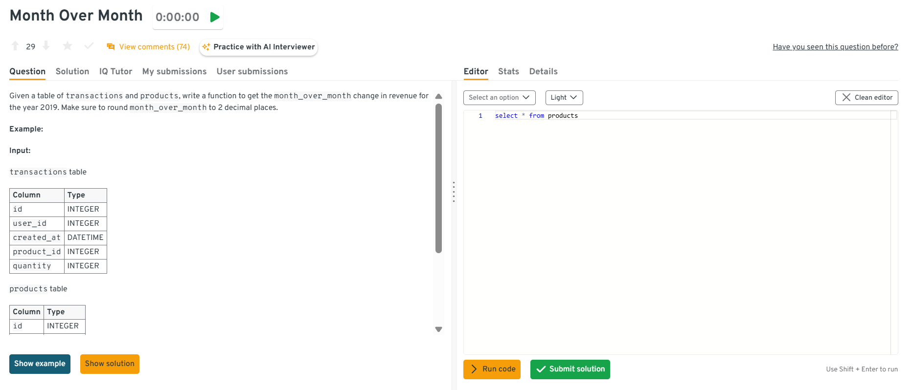
   Tip: Mention handling division by zero using NULLIF(employee_count, 0), since small details like this show production-ready thinking.

3. Find the month_over_month change in revenue for the year 2019.

   This question tests time-based windowing. To solve this, group revenue by month using DATE_TRUNC('month', order_date) and use LAG(SUM(revenue)) OVER (ORDER BY month) to compute the difference, then divide by the previous month’s revenue for a percent change.

   Tip: Clarify that you’d filter out the first month since it has no prior comparison, since such clean handling of edge cases always impresses interviewers.

   

   Explore the Interview Query dashboard that lets you practice real-world SQL and business analyst interview questions in a live environment. You can write, run codes, and submit answers while getting instant feedback, perfect for mastering business analyst problems across domains.

4. Write a query to identify customers who placed more than three transactions each in both 2019 and 2020

   This question tests your ability to apply conditional grouping and use multiple HAVING filters. Start by grouping transactions by customer_id and YEAR(order_date), then filter customers meeting the count threshold in both years. It’s a direct example of retention analysis and customer segmentation.

   Tip: Suggest using a pivot-style CTE or self-join of yearly aggregates, this shows comfort with data restructuring and analytical creativity.

5. Write a query to get the number of users who bought additional products after their first purchase.

   This is a classic way to identify repeat customers. The logic involves detecting a user’s first transaction, then counting subsequent purchases, which is perfect for understanding upsell effectiveness or lifecycle stages.

   Tip: Explain that you’d use MIN(order_date) or ROW_NUMBER() to identify the first purchase, showing awareness of multiple valid approaches signals flexibility.

6. Find the percentage of users that had at least one seven-day streak of visiting the same URL.

   This question checks your ability to define and detect behavioral patterns over time. The logic uses date differences or running sequences to detect consecutive visits, followed by an aggregate to count qualifying users and compute the percentage.

   Tip: Mention that you’d validate streak logic using test data first, which demonstrates analytical thoroughness and debugging discipline.

7. How would you aggregate three recipe tables to produce a single shopping list that sums the total mass of each ingredient?

   Combine the tables using UNION ALL, then GROUP BY ingredient and SUM(mass) to total quantities. Discuss unit standardization (grams vs. ounces) before summing and why UNION ALL preserves duplicates needed for a correct tally.

   Tip: Add that you’d ensure column names align before the union since mismatched schemas are a common real-world source of query errors.

8. Write SQL that returns the t-value and degrees of freedom to test whether category 9 products are cheaper on average than all others.

   This question combines SQL with statistical logic, assessing analytical depth. You’d calculate group means, variances, and counts for category 9 vs. others using aggregates, then compute the t-statistic via Welch’s formula.

   Tip: Note that you’d validate data distribution assumptions (e.g., excluding outliers) before testing, showing that you blend SQL with statistical judgment.

9. Which SQL logic samples every fourth record from a transaction table ordered by timestamp?

   This question tests window functions, row numbering, and ordered sampling logic. It’s about verifying whether you can generate and filter sequential records without relying on randomization. To solve it, order the transactions by date, assign a row number to each record, and then pick only every fourth one by filtering where that row number divides evenly by 4.

   Tip: Mention that ROW_NUMBER() or NTILE() functions keep order intact and prevent uneven distribution, which shows you understand deterministic sampling.

10. How would you retrieve the five projects with the highest budget-to-employee ratio, excluding projects with zero staff?

    This question tests joins, filtering, and ratio calculations. It evaluates your ability to combine employee counts with project budgets and compute meaningful efficiency metrics. You’d join the projects table with employee_projects, count employees per project, exclude those with zero staff, and divide each project’s budget by that count. Ordering by this ratio in descending order and limiting the output to five gives the required result. This mirrors real analyses where companies measure budget utilization across teams or departments.

    Tip: Mention using COUNT(DISTINCT employee_id) to avoid double counting and filtering early in the query to improve performance.

11. How would you identify the five users with the longest continuous daily-visit streaks?

    This question tests date arithmetic, window logic, and “gaps-and-islands” reasoning. The goal is to find consecutive-day user streaks, often used in engagement metrics or retention analysis. You’d assign each visit a sequential row number ordered by date, then subtract that from the actual date to form groups representing uninterrupted streaks. Counting visits within each group yields streak lengths; you then rank them and return the top five.

    Tip: Mention that you’d tie-break by earliest streak start to ensure deterministic results, which is a subtle but professional touch.

12. What SQL would categorize 2023 sales as Standard, Premium, or Promotional and then sum amounts by region?

    This question tests conditional logic (CASE statements) and grouped aggregation. It evaluates whether you can translate business rules into SQL conditions. You’d apply a CASE expression that labels each sale based on criteria such as region, month, or amount, then wrap that logic in a subquery and group by both region and category to get total sales. This kind of query powers dashboards where analysts segment sales performance for planning and reporting.

    Tip: Note that verifying category logic on a few sample rows first mirrors good QA habits analysts use before presenting insights.

13. How would you compute the share of lifetime revenue that occurred in the first and the last recorded years, rounded to two decimals?

    This question tests window functions, aggregation, and ratio calculations. The goal is to assess how well you summarize multi-year data while maintaining precision. You’d aggregate total revenue by year, identify the first and last years using MIN and MAX, sum those years’ revenue, divide by total lifetime revenue, and round the result. It’s a common analysis for measuring early- and late-stage performance in customer or product lifecycles.

    Tip: Explain that combining everything in one query avoids multiple scans and improves efficiency, showing that you think in terms of query optimization.

14. Which products have a list‐price higher than their own average transaction total, and how would you return product_id, product_price, and avg_transaction_total rounded to two decimals?

    This question tests aggregation with comparison logic. It’s about identifying products priced above their real-world selling average. You’d calculate each product’s average transaction value using a subquery or CTE, join it back to the products table, and filter for those where the listed price exceeds that computed average. Rounding both numeric columns to two decimals ensures clean presentation, as expected in business reporting.

    Tip: Point out that using window functions for the average instead of a subquery can simplify the query and make it more efficient on large datasets.

15. How many rows would result from an INNER, LEFT, RIGHT, and CROSS join between all ads and the top three most-popular ads?

    This question tests join behavior comprehension and dataset sizing logic. Interviewers use it to see if you understand how each join type affects row counts. You’d first create a top_ads CTE that selects the three most-popular campaigns, then run separate queries for each join type: an INNER join that returns only matching rows (three), LEFT and RIGHT joins that retain unmatched rows from one side, and a CROSS join that produces a Cartesian product of both sets. The key is explaining why row counts differ.

    Tip: Mention that estimating output size before executing heavy joins is part of good query hygiene, it prevents runtime surprises on large production data.

Advanced SQL questions are where interviews start to feel more analytical and performance-oriented. At this level, you’re not just writing queries, you’re designing efficient solutions for complex business problems.

Expect to see topics like subqueries, window functions (ROW_NUMBER(), RANK(), LAG()), indexing, and query optimization. You might be asked how to calculate running totals, identify user cohorts, or debug slow queries.

These questions test how deeply you understand SQL’s inner workings including what to write, and why you’d write it that way. Mastering this level shows you can handle real production-scale data and make smarter analytical decisions.

1. Compute cumulative users added daily with monthly resets

   This question tests advanced window framing and partition strategy on large time-series datasets. It evaluates your ability to compute per-month cumulative counts efficiently. To solve this, use SUM(1) OVER (PARTITION BY DATE_TRUNC('month', created_at) ORDER BY created_at ROWS BETWEEN UNBOUNDED PRECEDING AND CURRENT ROW) and cluster by created_at for better performance. In BI, this powers growth trend reporting with minimal recomputation.

   Tip: Mention verifying partition boundaries with sample outputs to show that you understand how frame definitions impact accuracy and performance.

2. Write a query to detect overlapping subscription periods

   This question tests interval logic and self-joins. It’s about identifying customers with overlapping subscriptions. Join subscriptions table to itself where one start_date falls between another’s start_date and end_date. Businesses use this for churn and double-billing prevention.

   Tip: Emphasize indexing both start_date and end_date for interval queries, this detail shows senior-level understanding of query performance on temporal data.

3. Count successful vs failed notification deliveries

   This question tests conditional aggregation for monitoring KPIs. Use SUM(CASE WHEN status = 'success' THEN 1 ELSE 0 END) and group by message type or platform. It’s common in operational analytics for reliability tracking.

   Tip: Mention that adding an UNION ALL validation layer comparing app logs with delivery DBs ensures end-to-end data integrity, since senior engineers think across systems, not tables.

4. Write a query to assign first-touch attribution in campaigns

   This question tests window functions and event sequencing for marketing analytics. Partition by user_id, order by event_time, and select ROW_NUMBER() = 1 to assign conversions to the first campaign touchpoint. It models marketing influence over user behavior.

   Tip: Highlight how you’d handle multi-channel overlap (e.g., paid vs. organic), showing business context awareness elevates technical answers.

5. Is click-through rate significantly related to human relevance ratings in search results, and what data will you return to test the hypothesis? 

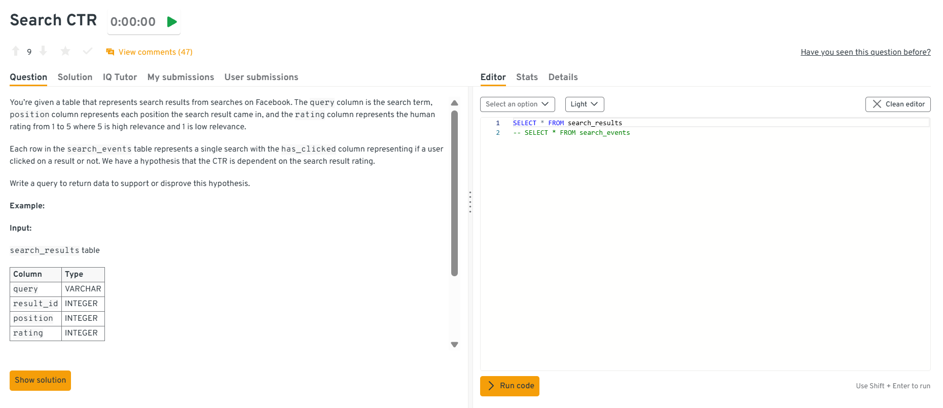
   Group search events by rating, calculate ctr = SUM(has_clicked)/COUNT(*), and return counts plus CTR per rating to enable a chi-square or logistic regression. Including confidence intervals or filtering by position helps control confounders. Strong answers mention that a rating-CTR relationship might be spurious without controlling for rank or query intent and suggest exporting raw aggregates for statistical testing offline.

   Tip: Emphasize linking SQL output to a downstream statistical test, showing that you understand how SQL fits within a full analytical workflow.

   

   Explore the Interview Query dashboard that lets you practice real-world SQL and business analyst interview questions in a live environment. You can write, run codes, and submit answers while getting instant feedback, perfect for mastering business analyst problems across domains.

6. How would you surface the five product pairs most frequently bought together by the same customer? 

   Aggregate each user’s distinct products into sets, explode them into unordered pairs via a self-join or ARRAY unnest, group by (least(p1,p2), greatest(p1,p2)), count co-occurrences, and pick the top five with p2 alphabetically first for ties. Efficient implementations pre-deduplicate (user_id, product_id) to cut pair generation size and may leverage approximate counts or partitioned tables for billion-row scale. Discussion of bloom filters, partition pruning, and batch processing shows senior-level thinking.

   Tip: Mention that deduplication before self-joins reduces computational cost dramatically and prevents inflated counts, which shows practical performance awareness.

7. Which January-2020 sign-ups moved more than $100 of successful volume in their first 30 days? 

   Join users (filtered to January-2020 signups) with payments twice—once as sender, once as recipient—keeping payment_state = 'success' and payment_date within 30 days of signup, sum amounts per user, and count those above $100. A union of the two roles preserves sign, and windowing by user_id plus a date filter ensures correctness. Good answers highlight indexes on (user_id, payment_date) and justify unions over OR conditions for planner efficiency.

   Tip: Point out that structuring filters before joins reduces scan size and improves performance, a practice interviewers look for at advanced levels.

8. What does the cumulative distribution of comment counts per user look like, by single-comment buckets? 

   First gather comment totals per user_id, then aggregate counts of users per num_comments, order the buckets, and compute a running fraction SUM(users)/total_users using a window function such as SUM(count) OVER (ORDER BY num_comments). If comment counts are sparse, generating a series with a left join fills gaps for smoother plots. The answer should mention why CUME_DIST() or PERCENT_RANK() can also be used and the importance of indexing the comments table on user_id.

   Tip: Add that validating cumulative sums against 100% helps ensure the distribution logic is correct and prevents silent miscounts in visualization outputs.

9. How would you report annual retention rates for a yearly-billed SaaS product? 

   Determine each customer’s cohort year via their first payment, then for every subsequent year compute SUM(is_renewed)/COUNT(*) within that cohort to get retention. A self-join or window function retrieves the first year, and a pivot produces a tidy year-by-year grid. Discussing churn definitions, handling partial years, and creating a composite index on (customer_id, payment_year) demonstrates scalable thinking.

   Tip: Mention that aligning cohorts by first billing date ensures fair comparisons across customers with different signup times. This kind of data hygiene is critical for retention accuracy.

10. Return the second-longest flight for each city pair

    This question tests ranking within groups. It’s specifically about normalizing city pairs (A-B = B-A), computing durations, and finding the 2nd-longest. To solve this, store sorted city names as city_a, city_b, compute duration_minutes, then apply ROW_NUMBER() OVER (PARTITION BY city_a, city_b ORDER BY duration_minutes DESC) and filter where rank=2. Airlines use this to plan backup aircraft allocations for long-haul routes.

    Tip: Note that indexing on (city_a, city_b) speeds up grouping for millions of flights and that precomputing duration avoids repeated calculations in large datasets.

Watch Next: Calculate Percentage of Revoked Job Postings | Advanced SQL Concepts

This session is an excellent resource for business analyst interview prep, especially for those looking to master SQL reasoning, optimization, and business interpretation in real interview settings.

In this advanced SQL mock interview, Sai Kumar (Lead Data Analyst at Carolina) walks through a real-world business analytics problem of calculating the percentage of revoked job postings within the last 180 days on a job board platform. He demonstrates how to use window functions, CTEs, ranking, and date filtering to derive meaningful metrics from messy data that goes beyond syntax—covering how to interpret the results, connect them to business outcomes, and propose new KPIs like revocation trends by location, job type, and employer trust score.

This is where SQL meets business. In this part of the interview, questions go beyond syntax and test your ability to translate real business problems into data queries.

You might be asked to analyze user behavior, track marketing campaign performance, or evaluate financial trends using SQL. The goal isn’t just to get the right output, but to think strategically, like what insights would you present to leadership, and how would they impact decisions?

These scenario-based questions are the most telling for business analyst roles because they reveal how well you connect data with outcomes. They’re a chance to show you’re not just a query writer, but a storyteller with data.

Read more: Top 25+ Data Science SQL Interview Questions

1. Write a query to find the number of confirmation message responses grouped by carrier and country for SMSs sent on February 28, 2020.

   Here, interviewers test your grasp of grouping and filtering in analytics queries. Filter the dataset using a WHERE clause for the specific date, then group by carrier and country, counting confirmation responses with COUNT() or conditional aggregation. This tests both SQL fundamentals and business reasoning, ensuring you can deliver clear insights for communication analytics. Edge cases may include missing response records or time zone mismatches.

   Tip: Mention using a CASE WHEN status = 'confirmed' THEN 1 END expression inside COUNT() to handle mixed statuses cleanly.

2. Given a table with event logs, find the top five users with the longest continuous streak of visiting the platform.

   This question evaluates your ability to use window functions for behavioral metrics. You can calculate consecutive visit streaks by comparing event dates with LAG() and resetting counts when a break occurs, then aggregate by user to find the longest streak. This problem tests analytical thinking, partition logic, and efficient event ordering, all key in product analytics pipelines.

   Tip: Emphasize handling edge cases where users skip days or have multiple events on the same day since both can break streak logic if not managed properly.

3. What SQL produces a pivot table of total sales by branch_id and year when sales are stored in separate yearly tables?

   The cleanest tactic unions the per-year tables into a CTE tagged with a year column, then leverages conditional aggregation: SUM(CASE WHEN year=2021 THEN total_sales END) AS sales_2021, etc. If the database supports dynamic SQL, a generated pivot scales to future years automatically. Good answers highlight the maintenance burden of one-table-per-year schemes and recommend folding data into a single partitioned fact table to simplify analytics and indexing.

4. How would you calculate a 3-day weighted moving average of product sales using weights 0.5, 0.3, 0.2 for days 0, -1, -2?

   A window function approach uses SUM(sales * weight) over a three-row frame: 0.5 * sales for the current row, 0.3 * LAG(sales,1), and 0.2 * LAG(sales,2). Filtering with WHERE LAG(sales,2) IS NOT NULL ensures that only rows with two predecessors are output. Explanations should mention choosing ORDER BY sale_date in the PARTITION BY product_id clause, discuss handling gaps in dates, and note that materializing daily sales in a pre-aggregated table avoids expensive on-the-fly computations.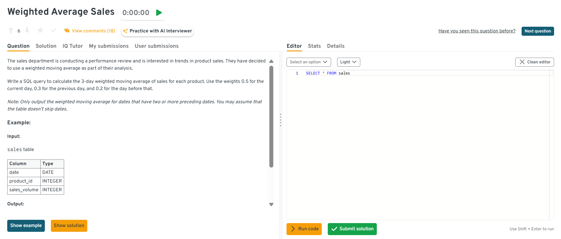

   

   Explore the Interview Query dashboard that lets you practice real-world SQL and business analyst interview questions in a live environment. You can write, run codes, and submit answers while getting instant feedback, perfect for mastering business analyst problems across domains.

5. Identify the top 3 marketing channels that generated the highest ROI last quarter.

   This question tests data aggregation and business impact analysis. You’d join the campaign_spend and sales_revenue tables on campaign_id, calculate ROI as (revenue - cost) / cost, and group by channel to find the top performers. This type of query evaluates your ability to connect SQL metrics to marketing strategy.

   Tip: Always mention how you’d handle missing spend or revenue data, showing you care about data accuracy, not just math.

6. Find customers who downgraded their subscription plan within 60 days of upgrading.

   This tests event sequencing and customer journey tracking. You’d use a self-join or window functions (LAG()/LEAD()) to compare each user’s consecutive subscription actions and calculate date differences. Filtering for users with an upgrade followed by a downgrade within 60 days reveals churn risk behaviors.

   Tip: Mention that filtering out trial plans or inactive users makes the analysis more meaningful to stakeholders.

7. Determine which products contributed the most to total revenue growth year-over-year.

   This question evaluates trend analysis and performance breakdowns. You’d aggregate revenue by product_id and year, calculate the percent change between years, and rank products by contribution to the total increase. This scenario directly connects SQL metrics to product strategy decisions.

   Tip: Explain that controlling for discontinued products or partial-year launches prevents misleading growth figures.

8. Identify cities with declining customer retention despite overall revenue growth.

   This question combines geographic segmentation with retention analytics. You’d compute retention rates per city using user activity data and compare year-over-year trends. Then, cross-reference with revenue data to find cities where revenue rose but retention fell. It’s a common case in regional performance reviews.

   Tip: Mention that you’d visualize these findings in a heat map, it shows you think about communicating insights, not just finding them.

9. Calculate the conversion funnel from website visit to purchase.

   This tests funnel analysis using conditional aggregation. You’d summarize counts for each stage (visits, add-to-cart, checkout, purchase) by user or session and compute conversion percentages step by step. This query demonstrates your understanding of user behavior flow and efficiency.

   Tip: Emphasize how you’d filter out bots or test sessions to ensure funnel metrics reflect real user behavior.

10. Measure how promotional discounts affected average order value (AOV).

    This question tests comparative analysis using CASE statements. You’d classify transactions as “discounted” or “non-discounted,” compute their average order values, and compare the two. This helps determine if promotions attract deal-seekers or drive genuine upsells.

    Tip: Suggest segmenting by customer type (new vs returning) to show a deeper, business-focused interpretation of the data.

While SQL skills prove you can work with data, your soft skills show how you work with people. Business analysts spend as much time explaining insights as they do writing queries, which means communication, collaboration, and clarity matter just as much as technical ability.

In this part of the interview, expect questions about how you’ve handled ambiguous requests, communicated technical findings to non-technical teams, or resolved data discrepancies. Interviewers want to see if you can bridge the gap between data and decision-making.

Tip: Use the STAR method (Situation, Task, Action, Result) to structure your answers, it keeps your responses focused, outcome-driven, and easy for interviewers to follow.

Read more: Top 32 Data Science Behavioral Interview Questions

1. Tell me about a time when you uncovered an important business insight using SQL.

   This question evaluates your analytical thinking and business impact.

   • Situation: While analyzing transaction data for a retail client, I noticed unusual spikes in refund rates during certain weekends.
   • Task: My goal was to identify the root cause and present actionable insights to reduce refund frequency.
   • Action: I queried the order and refund tables, joined them on order_id, and segmented results by product category and time. The SQL analysis revealed that a promotion on defective inventory caused the spike.
   • Result: The company pulled that product line early, preventing an estimated $120K in losses.

   Tip: Tie your SQL work directly to a measurable outcome, it shows that your analysis drives real decisions, not just dashboards.

2. Describe a time when a stakeholder gave you an unclear data request. How did you handle it?

   This tests your communication and problem-scoping skills.

   • Situation: A marketing manager asked for a report on “engagement,” but didn’t specify metrics or timeframe.
   • Task: I needed to clarify what “engagement” meant and ensure my SQL query measured what mattered.
   • Action: I scheduled a short sync, asked clarifying questions, and presented multiple metrics (sessions, click-throughs, and purchases) using CTEs for clarity.
   • Result: The manager chose click-through rate as the key KPI, and the resulting dashboard became a weekly performance tracker.

   Tip: Always confirm business definitions before writing SQL, because aligning expectations early saves hours of rework.

3. Talk about a time you identified and fixed a data inconsistency or quality issue using SQL.

   This question tests data validation and accountability.

   • Situation: Our monthly revenue report showed mismatched totals between the finance and sales dashboards.
   • Task: I needed to trace the issue and ensure accuracy before the next executive meeting.
   • Action: I used SQL joins and aggregation checks to trace duplicates in the transactions table. A missing DISTINCT in one CTE caused double-counting of partial refunds. After fixing it, I implemented validation checks comparing totals before and after aggregation.
   • Result: The corrected report reconciled both teams’ numbers and became a template for future QA queries.

   Tip: Explain not only how you fixed the issue but also how you prevented it from recurring — this shows process ownership.

4. Tell me about a time you had to explain SQL-based insights to a non-technical audience.

   This tests your ability to translate technical findings into business terms.

   • Situation: I built a SQL analysis to track customer churn patterns for the subscription team.
   • Task: The leadership team needed a clear explanation of why churn had increased without technical jargon.
   • Action: I visualized churn drivers by region and customer type, replacing SQL terms like “LEFT JOIN” or “window function” with plain explanations such as “comparing current and past month renewals.”
   • Result: The team approved a targeted retention campaign, reducing churn by 8% in two months.

   Tip: Simplify your story without diluting accuracy, since clarity wins more trust than complexity.

5. Describe a project where you used SQL to influence a business decision or strategy.

   This tests strategic impact and collaboration.

   • Situation: During a product launch analysis, leadership wanted to know whether the free trial feature increased conversions.
   • Task: I used SQL to compare conversion rates between trial users and direct signups, controlling for acquisition channel.
   • Action: After aggregating data and performing significance checks, I presented that trial users had 2.3× higher paid conversion but only in regions with localized onboarding.
   • Result: The finding led to expanding trial onboarding globally, improving conversions by 15%.

   Tip: Focus on the why behind your SQL, because when you connect data to business goals, it demonstrates executive-level analytical thinking.

Even experienced analysts trip up on SQL interviews, not because they lack skill, but because small oversights lead to big errors. Interviewers often watch for these patterns to see if you write clean, reliable, and business-friendly queries.

However, most of these mistakes are easy to fix once you know what to look for.

Read more: Common SQL Interview Mistakes and How to Avoid Them

Common SQL Mistakes and Why They Happen

Here’s a quick cheat sheet to help you identify common pitfalls and turn them into strengths during your interview.

Mistake	Why It Happens	Impact in an Interview
Forgetting to filter data correctly with WHERE	Rushing through problem setup	Leads to inaccurate results or inflated numbers
Using the wrong join type (INNER vs LEFT)	Misunderstanding table relationships	Causes missing or duplicated rows
Ignoring NULL values	Not accounting for incomplete data	Returns misleading averages or counts
Grouping without proper aggregation	Missing or incorrect GROUP BY logic	Results in syntax errors or inconsistent data
Overusing subqueries when joins are better	Lack of performance awareness	Slower queries, harder to debug
Writing unreadable or unformatted SQL	No indentation or aliasing	Hurts clarity, especially in panel interviews
Not testing queries with small datasets first	Jumping to full dataset immediately	Harder to trace logic errors or performance issues

Best Practices to Follow During SQL Interviews

The easiest way to stand out in SQL interviews is by writing clean, logical, and well-explained SQL. These best practices not only make your answers easier to follow but also show that you think like a professional analyst.

Here are some tried-and-true habits to follow:

Best Practice	Why It Works	Pro Tip
Write step-by-step queries	Helps you debug easily and explain logic clearly	Use CTEs (WITH statements) to organize your thoughts
Alias everything	Keeps queries readable and professional	Example: SELECT c.customer_id AS id instead of raw column names
Validate data assumptions	Shows analytical maturity	Always check for duplicates or NULLs before joining tables
Explain your reasoning out loud	Demonstrates communication and problem-solving	Talk through your joins, filters, and metrics
Use formatting and indentation	Reflects clean coding habits	Align keywords and clauses — readability counts
Double-check results	Prevents logical mistakes	Verify record counts or run sanity checks on outputs
Optimize only when needed	Shows balance between correctness and efficiency	Focus on clarity first, then mention possible optimizations

Tip: Interviewers care less about how fast you type and more about how clearly you think. If you can walk them through your logic, even when you make a mistake, you’ll leave a strong impression.

Preparation is what turns good analysts into confident interviewees. A solid SQL foundation is just the start, what really matters is how you practice, explain, and present your thinking under pressure.

Read more: How to Prepare for a Data Analyst Interview

Here’s a step-by-step preparation guide to help you get interview-ready:

• Review Core SQL Concepts

  Revisit the fundamentals like SELECT, WHERE, GROUP BY, JOIN, and HAVING. These make up the majority of SQL questions, even at intermediate levels.

  Tip: Practice rewriting the same query in different ways, it helps you spot more efficient solutions.

• Practice on Real Datasets

  Don’t limit yourself to textbook problems. Use datasets from Kaggle, Mode Analytics, or Interview Query’s SQL workspace to simulate real business challenges.

  Tip: Try answering open-ended questions like “Which customer segment is most profitable?” to mimic real analyst scenarios.

• Learn to Explain Your Logic

  Interviewers care as much about how you think as they do about your final answer. Be ready to describe your joins, filters, and reasoning step by step.

  Tip: Speak while you code, it mirrors the communication expected in real analytics teams.

• Master Joins and Aggregations

  Most interview challenges revolve around combining multiple tables and summarizing data correctly. Make sure you’re fluent in INNER, LEFT, RIGHT joins and GROUP BY logic.

  Tip: Always visualize relationships between tables before writing your query, it prevents logic errors.

• Practice Mock Interviews

  Run mock SQL sessions with peers or use platforms that simulate business case questions. This builds confidence and exposes weak areas early.

  Tip: Record yourself solving a query, reviewing your explanations helps polish clarity and timing.

• Build a Mini SQL Portfolio

  Create a few projects or case studies that show how you used SQL for real insights (sales analysis, retention tracking, marketing funnel analysis, etc.).

  Tip: Document your queries and findings in a clear format, it doubles as a great portfolio to share in interviews.

• Learn to Debug Efficiently

  Mistakes happen but the key is knowing how to identify and fix them fast. Learn to check joins, filters, and aggregations systematically.

  Tip: When stuck, test your logic on smaller chunks of data before running the full query.

• Use the Right Resources

  • Platforms: Interview Query Dashboard, Interview Query (SQL playlist), DataLemur, Mode SQL
  • Books: SQL for Data Analysis by Cathy Tanimura, Learning SQL by Alan Beaulieu
  • Courses: Coursera’s “SQL for Data Science,” DataCamp’s “SQL for Business Analysts”

  Tip: Choose interactive resources where you can write and test code, not just read syntax.

Acing the SQL interview is only part of the journey, the next step is knowing your worth. Business analysts with strong SQL skills are in high demand, and your ability to query, analyze, and communicate insights directly impacts your compensation.

Read more: Business Analyst Salary

Here’s how to approach salary discussions and long-term career growth with confidence:

1. Understand Typical Salary Ranges

   Compensation varies by company size, location, and your technical depth.

   • Entry-level business analyst: $70K–$90K (U.S.)
   • Mid-level analyst (2–4 years): $90K–$115K
   • Senior/lead analyst: $115K–$140K+

   Tip: Use tools like Interview Query Salary Explorer, Levels.fyi, and Glassdoor to benchmark your range before negotiating.

2. Know What Drives Your Value

   Analysts who can bridge business and technical skills, combining SQL with dashboarding tools, Python, or A/B testing often earn more.

   Tip: Mention how your SQL work impacted real metrics (e.g., reduced reporting time, improved retention analysis). That’s what hiring managers remember.

3. Evaluate the Entire Compensation Package

   Salary is just one part. Review bonuses, equity, 401(k), health coverage, and remote flexibility when comparing offers.

   Tip: Ask about learning budgets or certifications, many companies fund SQL or data science training.

4. Time Your Negotiation Right

   Negotiate after you’ve received an offer, not before. By that point, the company has already decided you’re a strong fit.

   Tip: Practice a calm, data-driven script like:

   “Based on my research and the role’s scope, I was expecting something closer to $X. Is there flexibility in the offer?”

5. Track Market Trends

   As of 2025-2026, demand for SQL-savvy business analysts continues to rise, especially in e-commerce, finance, and SaaS companies. Many firms now expect analysts to handle light data engineering or visualization work too.

   Tip: Stay current by following LinkedIn salary reports, Interview Query job market updates, and data analytics communities, they reveal shifts in demand early.

6. Plan for Career Growth

   Use your SQL foundation as a launchpad. Analysts who expand into data analytics, product analytics, or data science roles often see major salary jumps.

   Tip: Keep learning tools that complement SQL, like Python, Tableau, or dbt to future-proof your career.

What SQL concepts should business analysts focus on for interviews?

Focus on the essentials that mirror real-world work: SELECT, JOIN, GROUP BY, filtering with WHERE, window functions, and subqueries. Also understand data cleaning steps like handling NULL values or duplicates.

How do I explain my SQL query logic in an interview?

Walk the interviewer through your approach step-by-step: what the tables represent, why you’re joining them, and how each condition supports the question. Use simple phrasing like “First, I filtered by date; then, I grouped by user to count active sessions.”

What are common mistakes to avoid in SQL interviews?

Skipping filters, using the wrong join type, ignoring NULLs, or writing unreadable queries are common pitfalls. Always test your results with a small sample first.

What types of real-world scenarios are asked in business analyst SQL interviews?

Expect company-specific use cases like customer segmentation, churn analysis, sales reporting, or campaign performance tracking. These assess how you translate business problems into SQL logic. Practice domain-based questions (e.g., marketing, finance, e-commerce) to build context familiarity.

How can I prepare effectively for SQL interview questions?

Use interactive platforms like Interview Query, LeetCode (SQL), and Mode Analytics. Combine these with real datasets and mock interviews to simulate the pressure of a live test. Re-solve problems after a few days, spaced repetition cements SQL logic better than cramming.

What is the average salary for a business analyst with SQL skills?

In the U.S., business analysts with solid SQL proficiency earn between $75,000 and $120,000, depending on experience, industry, and location. Strengthen your case with measurable outcomes and show how your SQL insights improved KPIs or saved time.

How do SQL interviews differ for business analysts vs. data analysts?

Data analyst interviews lean more technical often covering Python, statistics, or visualization tools. Business analyst interviews, meanwhile, emphasize SQL for insights and storytelling while connecting query results to business impact.

What are the best resources to practice SQL interview questions?

The best way to practice SQL interview questions is by using interactive platforms where you can write and test queries directly. Start with the Interview Query SQL Question Bank for real interview problems, explore hands-on lessons with Mode Analytics SQL Tutorials, and sharpen your fundamentals through the LeetCode SQL Section. For deeper analytical context, read SQL for Data Analysis by Cathy Tanimura.

Preparing for a Business Analyst SQL interview is about understanding data, communicating clearly, and connecting every query to business value. By now, you’ve seen how interviewers test not only what you know but how you think: your ability to filter, join, aggregate, and interpret data with precision. You’ve also learned how to avoid common mistakes, prepare strategically, and negotiate confidently once the offer arrives.

With consistent practice and a thoughtful approach, you’ll walk into your SQL interview ready to do more than just write queries, you’ll be ready to tell stories with data and show exactly how your insights can drive results.

Helpful Interview Query Resources

Want to master SQL interview questions? Kick off your prep with our 14-Day SQL Study Plan and build hands-on confidence through real interview-style problems curated for quick practice.

Master CASE WHEN logic or GROUP BY filters with our step-by-step SQL Learning Path to go from basic joins to advanced optimization.

Then simulate the real pressure using Mock Interviews.