The Z and t test
The and tests are very basic tests that are most often used to test if means are equal/greater than/less than some hypothesized value. Generally, tests are used when the sample size is greater than 30, whereas -tests are used with sample sizes less than 30.
tests
Cheat Sheet
- Description: Tests if the mean is equal/less than/ greater than
- Statistic: (mean)
- Distribution: (normal)
- Sidedness: Either
- Null Hypothesis: (two-sided), (one-sided)
- Alternative Hypothesis: (two-sided), (one-sided)
- Test Statistic:
Description
The -test compares the mean of a sample (, also denoted as ) to some value, . It’s the go-to test for questions about the mean of some population. For example, if you had a sample of the GPA of students, you could run a -test to see if the students are doing well on average.
It assumes that the sample follows a normal distribution with some mean and variance .
In a two-sided -test, we want to check if . In a one-sided -test, we want to either test that or .
The mean of the sample is defined by the familiar notion of the arithmetic mean of a set of numbers: The test-statistic of the -test, called the -values or -score, is defined as
Where is the standard deviation of the assumed sample distribution . Most of the time, is not known in advance, so it is estimated through the sample standard deviation, .
This is because is an unbias estimator for , meaning that . By the way, this is why the term is included, because using the more intuitive constant of results in the bias estimator of , where .
Note how fits the general form of a test statistic we talked about in the previous section.
What is the decision function for the -test? Well, recall the general form of a decision function.
Remember, here refers to the sidedness of the test, which is 1 or 2, not the sample standard deviation.
Our test statistic is , and our assumed distribution is normal, so our cdf . So our decision function is:
Note: Throughout this course and in (almost all) real interviews, you will not be expected to calculate cdfs by hand. You can just describe what conclusions you would draw if you were given the value of
Example
Let’s go back to the question of student GPAs. Let’s say our sample is
and we want to know if students have at least a 3.0 on average. Our hypotheses would be:
Since there are samples here, we can use a one-sided -test to test these hypotheses. Here and so our -statistic is
If we set , since , we fail to reject . Thus, we do not have statistically significant evidence to say that the average student has a GPA higher than 3.0.
Tests
Note on notation
The -test is a bit of a notational nightmare to describe because is used to denote - The name of the test and distribution (we will use ) - The test statistic of the test (we will use ) - The notation of the -distribution (we will use ) - the pdf of the -distribution (we will use ) - the cdf of the -distribution (we will use ) To avoid confusion, we’ll use the notation denoted in parentheses above to refer to these elements in an unambiguous way.
Cheat sheet
- Description: Tests if the mean is equal/less than/ greater than for small samples ()
- Statistic: (mean)
- Distribution: ()
- Sidedness: Either
- Null Hypothesis: (two-sided), (one-sided)
- Alternative Hypothesis: (two-sided), (one-sided)
- Test Statistic:
Description
The -test is a modified version of the -test that allows for more conservative inferences when the sample size is small. Generally, a sample same size of is considered the cut-off between when to use a -test and a -test, samples with a size lower than 30. Thus in a situation where data collection is costly, like if we are collecting data via manual observation in a scientific experiment.
The only change to the decision function of the test compared to the is the assumed distribution of the sample. Instead of a normal distribution, it is assumed to follow a -distribution, which itself is a modification of the normal distribution.
The distribution does have a closed-form formula, but it is so complicated that it’s not very useful. It’s more important to focus on its shape and single parameter, , called the degrees of freedom. Because of this, the distribution can be called a -distribution with degrees of freedom. Importantly as gets large, the -distribution resembles a standard normal distribution more and more. That is
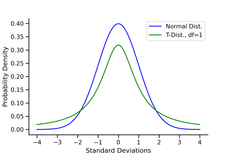
As you can see in the above animation, when the -distribution has very “long tails”. This represents the fact that in small sample sizes, we have a much higher probability of getting “extreme results” that deviate greatly from the mean. These long tails are how the -test controls for large sample sizes; they make it harder to reject compared to the -test. This fact can also be seen in the fact that the variance of the -distribution is , which is greater than 1 (the variance of the standard normal) but also converges to 1 as gets larger.
Because of this convergence, some professionals think it’s better to just always use a -test, since it will be equivalent to the -test for large sample sizes.
In the -test, is set to .
Example
Let’s only consider the GPAs of the first row of students in the -test
Here So Since , we still fail to reject and make the same conclusion as before.
In case you’re curious, if we used the entire sample, our -value from this -test would be about 0.2, just like the -test!
54%
CompletedYou have 35 sections remaining on this learning path.